- Captured On
- Source
- Linearization Near Critical Points | Unit IV: First-order Systems | Differential Equations | Mathematics | MIT OpenCourseWare
1 How can we get information about the trajectories of autonomous linear system without…
1.1 Front
How can we get information about the trajectories of autonomous linear system without…
determining them analytically or using a computer to plot them
1.2 Back
Analyzing what happens near critical points. We can do it linearizing the linear system at the critical points.
2 What does linearization mean of a non-linear system?
2.1 Front
What does linearization mean of a non-linear system?
2.2 Back
It’s an approximation near critical point by a linear system
3 What are the conditions for linearizate a non-linear system?
3.1 Front
What are the conditions for linearizate a non-linear system?
- \(x’ = f(x,y)\)
- \(y’ = g(x,y)\)
3.2 Back
You need to find their critical points, and for each point the functions \(f\) and \(g\) must be sufficiently differentiable.
4 Why high order terms in x and y can be neglected in a linearization of a non-linear system?
4.1 Front
Why high order terms in x and y can be neglected in a linearization of a non-linear system?
4.2 Back
Because the linearization is for points really close to critical points, so if the difference between critical point and another point is near \(0\), its higher values are really smaller
5 How can we get linearization using the Jacobian from multivariable linear approximation?
5.1 Front
How can we get linearization using the Jacobian from multivariable linear approximation?
- \(x’ = f(x,y)\)
- \(y’ = g(x,y)\)
Let be \((x_0, y_0)\) a critical point
Show the process
5.2 Back
We need to approximate \(f\) and \(g\) near \((x_0, y_0)\)
- \(\Delta x = x - x_0\)
- \(\Delta y = y - y_0\)
- \(\Delta f = f(x,y) - f(x_0,y_0)\)
- \({\displaystyle \Delta f \approx \biggl( \pdv{f}{x} \biggr)_0 \Delta x + \biggl(\pdv{f}{y} \biggr)_0 \Delta y}\)
As \(f(x_0,y_0) = 0\) (critical point)
\({\displaystyle f(x,y) \approx \biggl( \pdv{f}{x} \biggr)_0 \Delta x + \biggl(\pdv{f}{y} \biggr)_0 \Delta y}\)
We now make the change of variables
- \(x_1 = x - x_0 = \Delta x\)
- \(y_1 = y - y_0 = \Delta y\)
Getting the approximation of \(f\) and \(g\) computing before at \((x_0,y_0)\). The result is that in the neighborhood of the critical point \((x_0,y_0)\), the linearization of the system
- \({\displaystyle x_1’ = f(x,y) = \biggl( \pdv{f}{x} \biggr)_0 x_1 + \biggl(\pdv{f}{y} \biggr)_0 y_1}\)
- \({\displaystyle y_1’ = g(x,y) = \biggl( \pdv{g}{x} \biggr)_0 x_1 + \biggl(\pdv{g}{y} \biggr)_0 y_1}\)
In matrix notation, the linearization is therefore
\({\displaystyle \vb{x_1}’ = A \vb{x_1}}\), where \({\displaystyle \vb{x_1} = \begin{pmatrix}x_1 \\ y_1\end{pmatrix}}\) and \({\displaystyle A = \begin{pmatrix}f_x & f_y \\ g_x & g_y\end{pmatrix}_{(x_0, y_0)}}\)
the matrix \(A\) is the Jacobian matrix evaluated at the critical point \((x_0, y_0)\)
6 What is the Jacobian matrix for getting the linearization of this system?
6.1 Front
What is the Jacobian matrix for getting the linearization of this system?
- \(x’ = f(x,y)\)
- \(y’ = g(x,y)\)
Let be \((x_0, y_0)\) a critical point
6.2 Back
\({\displaystyle A = \begin{pmatrix}f_x & f_y \\ g_x & g_y\end{pmatrix}_{(x_0, y_0)}}\)
7 What is the general procedure for sketching the trajectories of non-linear system?
7.1 Front
What is the general procedure for sketching the trajectories of non-linear system?
7.2 Back
- Find all the critical points
- For each critical point
- Find the Jacobian matrix \(A\) of the linearized system
- Find the geometric type and stability of the linearized system
- Getting the eigenvalues
- If type is (saddle, node or spiral) (not star node or defective node)
- Getting the eigenvalues, direction on motion
- Sketch of trajectories near the critical point
- Mark all critical points in the \(xy\text{-plane}\), and sketch the trajectories around the critical points determined before
- Sketch in some other trajectories to fill out the picture
- Check compatibility with trajectories you have already sketched near critical points
- If you cannot sketch plausible trajectories, check possible mistakes
8 When does linearizing at critical points work to get trajectories of a non-linear system?
8.1 Front
When does linearizing at critical points work to get trajectories of a non-linear system?
8.2 Back
This method only works if the linearized system turns out to be a node, saddle, or spiral
9 When can we say that a system is structurally stable?
9.1 Front
When can we say that a system is structurally stable?
- \(x’ = f(x,y) = ax + by\)
- \(y’ = g(x,y) = cx + dy\)
9.2 Back
We say a system is structural if small changes in the system parameters (i.e., the constants that enter into the functions on the right hand side) do not changes the geometric type or stability of its critical points, or its limit cycles.
So, his system is structurally stable if it is a spiral, saddle, or node.
In cases of saddle or node, the eigenvalues are real and distinct, but not degenerate or star node. If coefficients changes a little, the eigenvalues will also change a little (see roots of the characteristic roots). So the new roots will still be real, and will have the same sign. Thus the changed system will still have the same geometric type and stability.
Similar interpretation could be done with complex eigenvalue with form \(r \pm si\), with \(r \gt 0\) and \(s \gt 0\), \(r \lt 0\) and \(s \gt 0\)
It’s easy to see with the \(TD\text{-diagram}\), if the system stays in the borderline, then and little change on the system parameters will change the type and the stability of the system.
10 When can we say what happen in a critical point in non-linear system?
10.1 Front
When can we say what happen in a critical point in non-linear system?
Without a doubt
10.2 Back
For an autonomous non-linear system, the linearized system correctly classifies the critical point if the linear system is a spiral node, a nodal source or sink, or a saddle.
11 What are the cases of borderline type of critical point on linearized non-linear system?
11.1 Front
What are the cases of borderline type of critical point on linearized non-linear system?
11.2 Back
- Eigenvalue pure imaginary: \(\lambda = 0 + si\), \(s \gt 0\)
- It corresponds to a center, so the trajectories are a family of concentric ellipses, centered at the origin
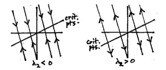
- Eigenvalue real and \(\lambda = 0\) (critical line)
- Shows a line of critical points (constant solutions), with all other trajectories being parallel ending up or away of at one of the critical points
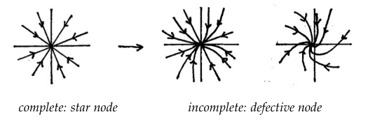
- One repeated real eigenvalue
- eigenvalue positive or negative
- eigenvector complete or defective
12 What does it happen if we change a little this system…
12.1 Front
What does it happen if we change a little this system…
- \(x’ = f(x,y) = ax + by\)
- \(y’ = g(x,y) = cx + dy\)
And the linearized system at critical point has eigenvalue pure imaginary
12.2 Back
In this case, this is a borderline geometric type, and it’s not stable. If we change a little the system, it will produce another type of system
From center trajectory to:
source spiral
sink spiral
center (\(\lambda=0 + 0i\))

13 What does it happen if we change a little this system…
13.1 Front
What does it happen if we change a little this system…
- \(x’ = f(x,y) = ax + by\)
- \(y’ = g(x,y) = cx + dy\)
And the linearized system at critical point has one eigenvalue real and the other is \(0\)
13.2 Back
In this case, this is a borderline geometric type, and it’s not stable
The solution of this linearized system has this form \(\vb{x} = c_1 \alpha_1 + c_2 \alpha_2 e^{\lambda t}\)

If the linearized system change a little, from the critical line to:
Unstable saddle
Critical line
Sink node

14 What does it happen if we change a little this system…
14.1 Front
What does it happen if we change a little this system…
- \(x’ = f(x,y) = ax + by\)
- \(y’ = g(x,y) = cx + dy\)
And the linearized system at critical point has only one repeated real eigenvalue
14.2 Back
In this case, this is a borderline geometric type, and it’s not stable.
Depending on whether eigenvalue is positive or negative, and whether the repeated eigenvalue is complete, or defective.
For example:
