Modes and the Characteristic Equation

Captured On

[2019-10-08 Tue 11:29]

Source

Modes and the Characteristic Equation | Unit II: Second Order Constant Coefficient Linear Equations | Differential Equations | Mathematics | MIT OpenCourseWare

1 In this system, when is the equilibrium point and what does it mean?

1.1 Front

In this system, when is the equilibrium point and what does it mean?

1.2 Back

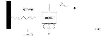
It’s at $x=0$, and it’s the point where the spring is relaxed, which means that it is exerting no force.

2 Which is the differential equation for this system?

2.1 Front

Which is the differential equation for this system?

2.2 Back

$m \ddot{x} = F_{\text{spr}} + F_{\text{ext}}$

3 Describe the model of the force of a spring

3.1 Front

Describe the model of the force of a spring

Looking for the simplest valid in general

3.2 Back

Is characterized by the fact that is depends only on position

• $x \gt 0 \implies F_{\text{spr}}(x) \lt 0$
• $x = 0 \implies F_{\text{spr}}(x) = 0$
• $x \lt 0 \implies F_{\text{spr}}(x) \gt 0$

Using the tangent line approximation

$F_{\text{spr}}(x) = -kx$, where $k \gt 0$

It’s call Hooke’s Law, and $k$ is called the spring constant

4 How can we model friction that it depends only on the velocity of the mass (no position)?

4.1 Front

How can we model friction that it depends only on the velocity of the mass (no position)?

4.2 Back

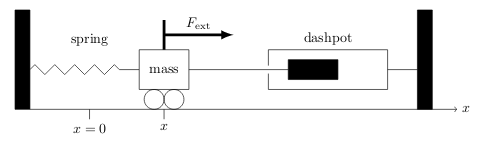
Using a dashpot, that is a cylinder filled with oil and a pistol moves through.

$F_{\text{dash}} = f(\dot{x})$, it opposes the velocity

• $\dot{x} \gt 0 \implies F_{\text{dash}} \lt 0$
• $\dot{x} = 0 \implies F_{\text{dash}} = 0$
• $\dot{x} \lt 0 \implies F_{\text{dash}} \gt 0$

$F_{\text{dash}}(\dot{x}) = -b \dot{x}$

This is called linear damping and $b$ is called the damping constant

5 What is a linear damping?

5.1 Front

What is a linear damping?

5.2 Back

It’s a simple model of friction that depends only on the velocity of the mass, not position

$F_{\text{dash}}(\dot{x}) = -b \dot{x}$, where $b$ is the damping constant

6 Write the differential equation which model this figure?

6.1 Front

Write the differential equation which model this figure?

6.2 Back

• $m \ddot{x} = F_{\text{spr}}(x) + F_{\text{damp}}(\dot{x}) + F_{\text{ext}}$
• $m \ddot{x} + b\dot{x} + kx = F_{\text{ext}}$

7 What is the Hooke’s law?

7.1 Front

What is the Hooke’s law?

7.2 Back

It’s the law which model the force of a spring which depends only on the position of the mass

$F_{\text{spr}}(x) = -k x$

8 Describe what is a general linear differential equation

8.1 Front

Describe what is a general linear differential equation

The generic form, and what means each part of the equation

8.2 Back

${\displaystyle a_x x^{(n)} + a_{n-1}x^{(n-1)} + \cdots + a_1\dot{x} + a_0 x = g(t)}$

• $a_k$ are the coefficients
  • May depend upon $t$, but not on $x$
  • If $a_n$ is not zero then the differential equation is said to be of order $n$
  • Are parameters of the system
• LHS of the equation represent the system
• RHS of the equation represent the input signal

If all coefficients are constant, this equation is called constant coefficient linear equation

9 Which the form of the equation of a second order homogeneous constant coefficient linear equation?

9.1 Front

Which the form of the equation of a second order homogeneous constant coefficient linear equation?

9.2 Back

$\ddot{x} + A\dot{x} + Bx = 0$

10 What is the model of a simple harmonic oscillator?

10.1 Front

What is the model of a simple harmonic oscillator?

In terms of $\omega$, and solutions

10.2 Back

It’s when the system is undamped, where it ODE is $m \ddot{x} + kx = 0$

${\displaystyle \ddot{x} + \frac{k}{m} x = 0}$

If we let $w = \sqrt{k/m}$, then $\ddot{x} + \omega^2 x = 0$

$x(t) = a x_1(t) + b x_2(t)$, where $x_1(t) = \cos(\omega t)$ and $x_2(t) = \sin(\omega t)$

Since the input is $0$ and the equation is linear, we can use superposition of solutions to get the general solution

$x(t) = a \cos(\omega t) + b\sin(\omega t) = A \cos(\omega t - \phi)$

Where $x(0) = a$ and $\dot{x}(0) = \omega b$, so you can solve (uniquely) for $a$ and $b$ to give any desired initial condition

11 What is the period of a nonzero solution $\ddot{x} + 4x = 0$

11.1 Front

What is the period of a nonzero solution $\ddot{x} + 4x = 0$

11.2 Back

Natural frequency $\omega_0 = \sqrt{k/m} = 2$

General solution, $x(t) = c_1 \cos(2t) + c_2 \sin(2t) = A \cos(2t - \phi)$ (In both rectangular and phase-amplitude form)

So, the period $P = \frac{2\pi}{\omega} = \frac{2 \pi}{2} = \pi$

12 How can we solve this general second ODE?

12.1 Front

How can we solve this general second ODE?

$m\ddot{x} + b \dot{x} + kx = 0$

Explain the process to get a solution

12.2 Back

• It’s similar to $\dot{x} +kx=0$ which solution is $x = e^{-kt}$
• We’ll be optimistic and try for exponential solutions
  • $x(t) = e^{rt}$
• Plug into the ODE
  • $x = e^{rt}$
  • $\dot{x} = re^{rt}$
  • $\ddot{x} = r^2e^{rt}$
• $m\ddot{x} + b\dot{x} + kx = 0 \implies (mr^2 + br + k)e^{rt} = 0$
• As $e^{rt} \neq 0$ for any $t$, we can divide up this equation by $e^{rt}$
  • $x(t) = e^{rt}$ is a solution always that $r$ satisfies the characteristic equation $mr^2 + br +k = 0$
  • The characteristic polynomial $p( r) = mr^2 + br + k$
• Solving the characteristic equation we’ll get 2 solutions $x_1(t) = e^{r_1t}$ and $x_2(t) = e^{r_2t}$
• By superposition, the linear combination of independent solutions
  • $x(t) = c_1x_1(t) + c_2 x_2(t) = c_1e^{r_1t} + c_2 e^{r_2t}$

13 What is the characteristic equation for solving second ODE?

13.1 Front

What is the characteristic equation for solving second ODE?

$m \ddot{x} + b\dot{x} + kx = 0$

13.2 Back

In a homogeneous second order ODE, we’ll be optimistic and say that $x(t) = e^{rt}$ is a solution for this ODE. Plugging in the ODE

$(mr^2 + br + k)e^{rt} = 0$

That’s the characteristic equation

14 What is the characteristic polynomial for General $n\text{-th}$ ODE?

14.1 Front

What is the characteristic polynomial for General $n\text{-th}$ ODE?

$a_nx^{(n)} + \cdots + a_1\dot{x} + a_0 x = 0$

14.2 Back

$p( r) = a_n(r^n) + \cdots + a_1 r + a_0$

15 How can we get a specific solution from IVP on second order ODE?

15.1 Front

How can we get a specific solution from IVP on second order ODE?

Initial conditions: $x(0)$ and $\dot{x}(0)$

15.2 Back

After getting the characteristic equation, you will get 2 possible solutions. Solving this system of equations

• $x(0) = c_1 e^{r_1 t} + c_2 e^{r_2 t}$
• $\dot{x}(0) = r_1 c_1 e^{r_1t} + r_2 c_2 e^{r_2t}$

16 What is a modal solution?

16.1 Front

What is a modal solution?

16.2 Back

It’s a solution of the form $x(t) = ce^{rt}$ to the homogeneous constant coefficient linear equation

${\displaystyle a_x x^{(n)} + a_{n-1}x^{(n-1)} + \cdots + a_1\dot{x} + a_0 x = 0}$

17 What is a mode of the system?

17.1 Front

What is a mode of the system?

17.2 Back

$e^{rt}$ is a mode of the system where $x(t) = e^{rt}$ is a solution to the homogeneous constant coefficient linear equation

${\displaystyle a_x x^{(n)} + a_{n-1}x^{(n-1)} + \cdots + a_1\dot{x} + a_0 x = g(t)}$

18 Can I use the solution $e^{rt}$ for any linear equation?

18.1 Front

Can I use the solution $e^{rt}$ for any linear equation?

Where $r$ is a root of the characteristic polynomial

18.2 Back

No, this only works for homogeneous constant coefficients linear equations

${\displaystyle a_x x^{(n)} + a_{n-1}x^{(n-1)} + \cdots + a_1\dot{x} + a_0 x = 0}$

Where $a_i$ are constants.

It does not work for non-constant coefficient or inhomogeneous or nonlinear equations

19 How could be the roots of the characteristic polynomial?

19.1 Front

How could be the roots of the characteristic polynomial?

19.2 Back

• Roots can be real or non-real complex numbers
• Roots can also be repeated

20 How are the modal solutions where roots of characteristic polynomial are real?

20.1 Front

How are the modal solutions where roots of characteristic polynomial are real?

In a second order constant coefficients linear equation

20.2 Back

The modal solutions are $x_1(t) = e^{r_1 t}$ and $x_2(t) = e^{r_2 t}$

21 How are the general solution where roots of characteristic polynomial are real?

21.1 Front

How are the general solution where roots of characteristic polynomial are real?

In a second order constant coefficients linear equation

21.2 Back

The general solution is found by superposition

$x(t) = c_1 x_1(t) + c_2 x_2(t) = c_1 e^{r_1 t}+ c_2 e^{r_2t}$

22 How are the modal solution where roots of characteristic polynomial are non-real complex?

22.1 Front

How are the modal solution where roots of characteristic polynomial are non-real complex?

In a second order constant coefficients linear equation

22.2 Back

• $r_1 = a + ib \implies z_1(t) = e^{(a + ib)t}$
• $r_2 = a - ib \implies z_2(t) = e^{(a - ib)t}$

Where $z$ indicate the functions are complex valued, but both will produces the same basic solutions because of $\cos(bt) = \cos(-bt)$ and $-\sin(bt) = \sin(-bt)$

Applying the superposition solution, we won’t get any new solution

23 How does we expect solutions in DE when has real coefficients?

23.1 Front

How does we expect solutions in DE when has real coefficients?

23.2 Back

We’re expecting real value solutions

24 What is the Real Solution Theorem?

24.1 Front

What is the Real Solution Theorem?

Let $z(t)$ be a complex-valued solution to a second order constant coefficients linear equation, where all coefficients are real

Give a proof

24.2 Back

The real and imaginary parts of $z$ are also solutions

If $z(t) = u(t) + i v(t)$, we can build the table

\begin{align*} k] \qquad z &= u + iv \\\ b] \qquad \dot{z} &= \dot{u} + i\dot{v} \\\ m] \qquad \ddot{z} &= \ddot{u} + i\ddot{v} \\\ \end{align*}

Summing the coefficients ($z$ is solution of the homogeneous DE)

$(m \ddot{u} + b \dot{u} + ku) + i(m\ddot{v} + b\dot{v} + kv) = 0$

The only way the sum can be zero is for both of them to be zero. That is, both $u$ and $v$ are solutions

25 What is the general solution if roots of characteristic polynomial are complex?

25.1 Front

What is the general solution if roots of characteristic polynomial are complex?

• $r_1 = (a + ib)$
• $r_2 = (a - ib)$

25.2 Back

Using the Real Solution Theorem, where modal are

• $z_1(t) = e^{(a + ib)t} = e^{at}(\cos (bt) + i\sin(bt))$
• $z_2(t) = e^{(a - ib)t} = e^{at}(\cos (-bt) + i\sin(-bt))$

From $z_1(t)$, the real solution is (using superposition)

$x(t) = c_1 e^{at} \cos(bt) + c_2 e^{at} \sin(bt) = e^{at} (c_1 \cos (bt) + c_2 \sin (bt)) = Ae^{at}\cos(bt - \phi)$

From $z_2(t)$, the real solution is

$x(t) = c_1 e^{at} \cos(-bt) + c_2 e^{at} \sin(-bt) = e^{at} (c_1 \cos (bt) - c_2 \sin (bt)) = Ae^{at}\cos(bt - \phi)$

Up to a sign these are the same basic solutions as was obtained from $z_1$, so $z_2$ would have work just as well

We don’t need to get both real solutions