- Captured On
- Source
- First Order Autonomous Differential Equations | Unit I: First Order Differential Equations | Differential Equations | Mathematics | MIT OpenCourseWare
1 What is an autonomous first order differential equation?
1.1 Front
What is an autonomous first order differential equation?
1.2 Back
There are (in general) nonlinear equations of the form \(\dot{x} = f(x)\)
The word autonomous means self governing and indicates that the rate of change of \(x\) is governed by \(x\) itself and it not dependent of time.
2 What differences are there between general and autonomous first order ODE?
2.1 Front
What differences are there between general and autonomous first order ODE?
2.2 Back
- General first order ODE: \(\dot{x} = f(x,t)\)
- Autonomous first order ODE: \(\dot{x} = f(x)\) (not dependent on time), in general nonlinear
3 What are the properties of autonomous first order ODE?
3.1 Front
What are the properties of autonomous first order ODE?
3.2 Back
\(\dot{x} = f(x)\)
- Model conditions which are constant in time, though they may depend on the current value of \(x\)
- They are separable
- They can be hard to integrate
- We can say a lot about them without solving them
- Time invariant
- if \(y(t)\) is a solution then is \(y(t - t_0)\) for any value of \(t_0\)
4 What kind of qualitative information can get from autonomous first order ODE?
4.1 Front
What kind of qualitative information can get from autonomous first order ODE?
In population models and physical models
4.2 Back
- Population models
- Stabilizes?
- Crashes?
- Explodes?
- Physical models
- Self correcting?
- Fall apart?
5 What are the equilibrium equations in the autonomous first ODE?
5.1 Front
What are the equilibrium equations in the autonomous first ODE?
\(\dot{y} = f(y)\)
5.2 Back
Constants solutions \(y(t) = y_0\) where \(y(y_0) = 0\)
Your are looking for points (critical points), where \(\dot{y} = 0\). It’s solutions are constants and you can draw isoclines where \(m = 0\) (nullcline)
6 How can we draw a isoclines graph for an autonomous first ODE?
6.1 Front
How can we draw a isoclines graph for an autonomous first ODE?
\(\dot{y} = f(y)\)
6.2 Back
All constant solutions are horizontal straight lines
At critical points \(\dot{y} = f(y_0) = 0\), are nullcline (Equilibrium solutions)
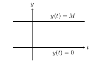
As, integral curves cannot cross solutions, they cannot cross constant solution neither.
To draw another isoclines you can draw a graph of \(f(y)\) as a function of \(y\). And check where the slope is positive or negative

Draw some intermediate isocline between constant solutions

7 What are the critical point in a autonomous first ODE?
7.1 Front
What are the critical point in a autonomous first ODE?
\(\dot{y} = f(y)\)
7.2 Back
The value of the equilibrium solutions, i.e., values \(y_0\) where \(f(y_0) = 0\)
8 What is a stable equilibrium in a autonomous first ODE?
8.1 Front
What is a stable equilibrium in a autonomous first ODE?
\(\dot{y} = f(y)\)
8.2 Back
An equilibrium solution where all nearby solution curves tend towards it
9 What is an unstable equilibrium in a autonomous first ODE?
9.1 Front
What is an unstable equilibrium in a autonomous first ODE?
\(\dot{y} = f(y)\)
9.2 Back
An equilibrium solution where all nearby solution curves tend away from it
10 What is a logistic curves (S-curve) in a autonomous first ODE?
10.1 Front
What is a logistic curves (S-curve) in a autonomous first ODE?
\(\dot{y} = f(y)\), in a logistic population model
10.2 Back
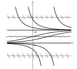
The solutions that start in an unstable equilibrium and go asymptotically to an stable equilibrium
11 What is carrying capacity in the logistic model?
11.1 Front
What is carrying capacity in the logistic model?
\(\dot{y} = f(y)\)
11.2 Back
The stable equilibrium that all (positive) populations approach asymptotically

12 What is a Logistic Population Model?
12.1 Front
What is a Logistic Population Model?
Use the simplest line, \(k\) declines as \(y\) increases
12.2 Back
It’s an autonomous first ODE, \(\dot{y} = f(y)\), where takes into account the limits the environment imposes on population growth
\(\dot{y} = k(y) \cdot y\)
The growth rate start at \(k_0\) and decrease as \(y\) increases until \(y = M\), where the growth rate is 0 and then is negative
\(k = k_0(1 - y/M)\)
\(\dot{y} = k_0(1 - y/M)y = f(y)\)
13 Where are the stable and unstable critical points in this graph?
13.1 Front
Where are the stable and unstable critical points in this graph?
13.2 Back
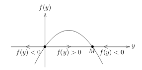
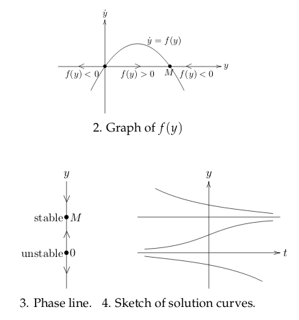
- Critical points at \(f(y) = 0\)
- Stable critical point: \(y = M\), \((0,M)\) (Arrows toward to that point)
- Unstable critical point: \(y = 0\), \((0,0)\) (Arrows away from that point)
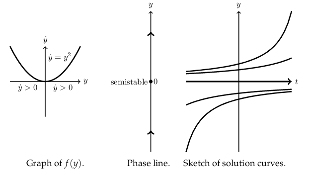
If there are 2 arrows at the same direction between a critical point. It’s stable in one direction, but unstable on the other. It’s called semi stable
14 This critical point is stable or unstable?
14.1 Front
This critical point is stable or unstable?
14.2 Back
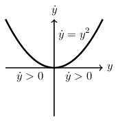
It’s stable from solutions below \(y = a\), but unstable for solution above \(y = a\)
It’s semi stable critical point
15 What is a phase line for a autonomous first ODE?
15.1 Front
What is a phase line for a autonomous first ODE?
\(\dot{y} = f(y)\)
15.2 Back
It’s a vertical line (\(y\text{-axis}\)) where there are critical point marked (\(f(y) = 0\))
In each interval delimited by critical points draw an upward pointing arrow if \(f(y) > 0\) (\(\dot{y} >0\)) and downward pointing arrow if \(f(y) < 0\) (\(\dot{y}<0\))
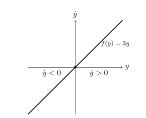
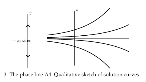
Also phase line tell you what happens to the integral curves in the long-run, as \(t \to \infty\)
16 What are the steps to give a qualitative sketch of curve solution?
16.1 Front
What are the steps to give a qualitative sketch of curve solution?
for an autonomous first ODE
\(\dot{y} = f(y)\)
16.2 Back
- Find the critical points
- Plot graph of \(f(y)\) and determine where \(\dot{y}\) is positive and negative
- Draw the phase line and find the stability of the critical points
- Sketch the solution curves
17 What that mean that solutions can be shifted in Time?
17.1 Front
What that mean that solutions can be shifted in Time?
17.2 Back
It refers to autonomous equation \(\dot{y} = f(y)\), where the direction field is constant in the horizontal direction. That means that conditions represented by the ODE are constant in time.
Any solution translated horizontally to another time is also a solution
A “time translate” of a function \(y(t)\) is a function \(y(t - t_0)\); the graph is shifted horizontally (to the right) by \(t_0\) units
18 What means a “time translate” function of \(y(t)\) to \(y(t - t_{0})\)?
18.1 Front
What means a “time translate” function of \(y(t)\) to \(y(t - t_{0})\)?
18.2 Back
It’s mean that the graph of \(y(t - t_0)\) is shifted horizontally to the right by \(t_0\) units
19 Can solutions have a local maximum?
19.1 Front
Can solutions have a local maximum?
On autonomous first ODE, \(\dot{y} = f(y)\)
19.2 Back
No
Suppose \(y(t_0) = y_0\) and \(\dot{y_0} = 0\), then there is an equilibrium solution \(y(t) = y_0\). By the existence and uniqueness theorem this is the only solution \(y(t_0) = y_0\).
Non-constant solutions never have derivative equal to \(0\) (they don’t have any local maxima or minima)
But, constant functions have local maxima, just not strict local maxima. All values of this constant solution are maximum values, but no value of the function is larger than nearby values.
20 When do non constant solutions of the autonomous ODE have inflection points?
20.1 Front
When do non constant solutions of the autonomous ODE have inflection points?
\(\dot{y} = f(y)\)
20.2 Back
When \(f’(y) = 0\), \({\displaystyle \dv{y}{t} = f(y) \implies \dv[2]{y}{t} = f’(y) \dv{y}{t}}\)
Inflection point where \({\displaystyle \dv[2]{y}{t} = 0}\), but his happens when
- \(\dot{y} = 0\) (Constant solution which have no inflection points)
- \(f’(x) = 0\)